Skip to content

Simulations & Solvers

269 Topics 801 Posts

FDTD, Low-Frequency, Neuron, Mode-Matching, Flow, Acoustics, etc...

Subcategories


  • FDTD, Low-Frequency, Neuron, Mode-Matching, Flow, Acoustics, etc...

    16 39
    16 Topics
    39 Posts
    G
    Hi, I'm trying to simulate a synapse between two identical neuron models, imported from the same .hoc file. I set the simulation as follow (see screenshot): -both neuron have the same HOC Model Settings -The first neuron "L23_PC_cADpyr229_1", pre-synaptic, has an IClamp on its soma -The second neuron "L23_PC-cADpyr229_2", post-synaptic, has a Exp2Syn point process on dendrite 9 -The network connection was created drag & dropping the first neuron's model and the Exp2Syn point process of the second neuron in the network connection settings [image: 1778756649765-f7472fbe-2fe9-4244-9297-34d7a1f29c16-image.png] If I try to run the simulation I get the error messages: Simulation : [Error] Failed to create neuron group ids. Error : Failed to write the input file Error : Unable to start simulation: failed to write input files. How can I solve this error? I already tried using different neurons from different .hoc files. Thank you in advance
  • FDTD Timestep

    2
    0 Votes
    2 Posts
    1k Views
    M
    Hi, As FDTD is a time-domain based method, implementing LF sources with this method is quite challenging. It would need a very (very) long simulation's time, without any assurance of reaching the correct convergence level at the end - furthermore if your simulation has a certain amount of MCells. For input signal with frequency components below the MHz, LF approach is the only solution that would give you quick and accurate results. I would thus advice you to (1) get the current profile along time, and (2) do a fft so as to get the current's magnitude for each of the frequency components. Then, (3) perform several LF simulations for each of the frequency/magnitude obtained during step (2). Best
  • Maximum Cell Count

    10
    0 Votes
    10 Posts
    5k Views
    J
    thanks. It works if I lower it to 55khz, but not if I lower it to 2kHz.
  • Material anisotropy along a curve?

    4
    0 Votes
    4 Posts
    2k Views
    M
    Something to get started to create an anisotropic conductivity tensor for S4L from solving a Poisson equation with boundary conditions (running an EM simulation and using its potential). Once the field is created in the analysis tab it can be used as a part of a new EM simulation for any material selected to have inhomogeneous and anisotropic properties. import numpy as np import s4l_v1.document as document import s4l_v1.model as model import s4l_v1.simulation.emlf as emlf from s4l_v1 import ReleaseVersion, Unit from s4l_v1.model import Vec3, Translation, Rotation import s4l_v1.units as units import s4l_v1.analysis as analysis import XCoreModeling def CreateMockAnisotropicConductivity(sim): # Transversal and longitudinal sigmas sigma1 = 3.0 sigma2 = 1.0 # here conductivity has 6 component (anisotropic tensor) results = sim.Results() p = results["Overall Field"].Outputs["EM Potential(x,y,z,f0)"] p.Update() e = results["Overall Field"].Outputs["EM E(x,y,z,f0)"] e.Update() e_field = e.Data.Field(0) nc = e.Data.Grid.NumberOfCells print "E Field shape", e_field.shape print "Number of Cells", nc # E Field shape (nc, 3) - Cell centered # Calculate sigma on cell centers print "Calculate anisotropic sigma values" sigma_wm = np.zeros([nc,6]) # 6 unique values # tensor component indexing for solver iu3 = (np.array([0, 1, 2, 0, 1, 0], dtype=np.int64), np.array([0, 1, 2, 1, 2, 2], dtype=np.int64)) for idx, val in enumerate(e_field): tmp = np.zeros([3,3], dtype=np.complex) tmp[0] = val if (not np.isnan(val).any() and np.inner(val, val) != 0): P = np.dot(tmp.T, tmp) / np.inner(val,val) else: P = np.full((3, 3), 0, dtype=np.complex) sigma_tensor = sigma1*P + sigma2*( np.identity(P.shape[0]) - P ) sigma_wm[idx] = sigma_tensor[iu3].real sigma_swapped = sigma_wm[:,[0,1,2,3,5,4]] # Fix bug where yz and xz were swapped tensor_conductivity = analysis.core.DoubleFieldData() tensor_conductivity.NumberOfSnapshots = 1 tensor_conductivity.NumberOfComponents = 6 tensor_conductivity.Grid = e.Data.Grid.Clone() tensor_conductivity.ValueLocation = analysis.core.eValueLocation.kCellCenter tensor_conductivity.SetField(0, sigma_swapped) #sigma_wm) # Fix bug where yz and xz were swapped tensor_conductivity.Quantity.Name = 'Anisotropic Conductivity From E Field' tensor_conductivity.Quantity.Unit = analysis.core.Unit('S/m') producer_t = analysis.core.TrivialProducer() producer_t.SetDataObject(tensor_conductivity) producer_t.Name = 'Anisotropic Conductivity' document.AllAlgorithms.Add(producer_t)
  • Inhomogenous anisotropic electrical conductivity

    6
    0 Votes
    6 Posts
    3k Views
    M
    @montanaro said in Inhomogenous anisotropic electrical conductivity: Hi yes this is possible in the latest release of Sim4Life, however there isn't a good tutorial for it at the moment (I'll help prepare one). Essentially what is needed is to create a Trivial Producer (an artificial field distribution in the Analysis tab) via Python that has 6 components, representing the symmetric anisotropic tensor values ordered in such a way: xx, yy, zz, xy, xz, yz. Each component should have the full anisotropic values that will be interpolated into the simulation grid. This trivial producer must be assigned the correct units of S/m (this is all handled via a Python script). Once that is done, then in your EM simulation you can assign these values to any given material: Materials -> Electric Conductivity: Anisotropic, Inhomogeneous -> Data Origin: Analysis Output -> Then you can select your field. I'll hopefully find some time to update this comment here with a sample script. Here's a sample script I found to import VTI data and convert it to a Trivial producer in the correct format. Let me know if anything is not clear. # -*- coding: utf-8 -*- import os import numpy as np import vtk from vtk.numpy_interface import dataset_adapter as dsa import XCoreModeling import XPostProcessor fp = r"D:\Users\sample\path" fn = "sample.vti" f = os.path.join(fp, fn) reader = vtk.vtkXMLImageDataReader() reader.SetFileName(f) reader.Update() img = dsa.WrapDataObject(reader.GetOutput()) dxx = img.PointData['Dxx'] dyy = img.PointData['Dyy'] dzz = img.PointData['Dzz'] dxy = img.PointData['Dxy'] dyz = img.PointData['Dyz'] dxz = img.PointData['Dxz'] dims = img.VTKObject.GetDimensions() origin = img.VTKObject.GetOrigin() spacing = img.VTKObject.GetSpacing() # scale to meters scale = XCoreModeling.GetActiveModel().LengthUnits.ToUnit(XPostProcessor.Unit.Meter) origin = [scale*origin[0], scale*origin[1], scale*origin[2]] spacing = [scale*spacing[0], scale*spacing[1], scale*spacing[2]] grid = XPostProcessor.UniformGrid() grid.SetUnit(0, XPostProcessor.Unit.Meter) # note meters here grid.SetUnit(1, XPostProcessor.Unit.Meter) grid.SetUnit(2, XPostProcessor.Unit.Meter) # create dual grid, so we can assign point data from image as cell centered data grid.SetDimensions(dims[0]+1, dims[1]+1, dims[2]+1) grid.SetOrigin(origin[0]-0.5*spacing[0], origin[1]-0.5*spacing[0], origin[2]-0.5*spacing[0]) grid.SetSpacing(spacing[0], spacing[1], spacing[2]) assert grid.NumberOfCells == dxx.shape[0] sigma = np.zeros([grid.NumberOfCells,6]) sigma[:,0] = dxx sigma[:,1] = dyy sigma[:,2] = dzz sigma[:,3] = dxy sigma[:,4] = dyz sigma[:,5] = dxz aniso_cond = XPostProcessor.DoubleFieldData() aniso_cond.Grid = grid aniso_cond.NumberOfSnapshots = 1 aniso_cond.NumberOfComponents = 6 aniso_cond.ValueLocation = XPostProcessor.eValueLocation.kCellCenter aniso_cond.SetComponentLabel(0, "Dxx") aniso_cond.SetComponentLabel(1, "Dyy") aniso_cond.SetComponentLabel(2, "Dzz") aniso_cond.SetComponentLabel(3, "Dxy") aniso_cond.SetComponentLabel(4, "Dyz") aniso_cond.SetComponentLabel(5, "Dxz") aniso_cond.SetField(0, sigma) aniso_cond.Quantity.Name = 'Anisotropic Conductivity From DTI (use for Bone)' aniso_cond.Quantity.Unit = XPostProcessor.Unit('S/m') producer_t = XPostProcessor.TrivialProducer() producer_t.SetDataObject(aniso_cond) producer_t.Description = 'Anisotropic Conductivity' XPostProcessor.AlgorithmRegistry().AddAlgorithm(producer_t)
  • This topic is deleted!

    1
    1
    0 Votes
    1 Posts
    2 Views
    No one has replied
  • Multidomain mesh not shown in mesh tools

    3
    0 Votes
    3 Posts
    2k Views
    C
    The multidomain mesh is currently not available for Sim4Life light, that's why the relevant button does not appear in the ribbon.
  • Using Multiple GPUs does not improve simulation time

    1
    0 Votes
    1 Posts
    932 Views
    No one has replied
  • Linear system solver could not determine the solution

    1
    0 Votes
    1 Posts
    797 Views
    No one has replied
  • Choosing current instead of voltage in electrodes

    1
    1 Votes
    1 Posts
    798 Views
    No one has replied
  • Voxel-wise initial conditions for Thermal Simulations

    2
    0 Votes
    2 Posts
    1k Views
    M
    Hi, In transient thermal simulation, several ways of defining initial temperatures distribution are available (as detailed in the Manual, section 2.8.2.5). In your case, either 'steady state' or 'continue simulation' can allow you to avoid those 30 min with no EM sources. Here an example of process: (1) Run a first thermal simulation with only the human model and its proper thermal features, until reaching the required steady-state. This simulation would be the initialization of all your thermal simulations. (2) Create a 2nd simulation in which the 'Material' is defined as for the first one and use the 'Continue Simulation' option. You would also need to define the 'Snapshot', meaning at what time of the first simulation you are considering the initial temperatures (take care in case of non-convergence). EM sources can then be directly applied at 0 second. For ensuring accuracy, I would advice you to keep the same grid for all your thermal simulations. Best, Mélina
  • Break of continuity on E-field

    1
    5
    0 Votes
    1 Posts
    628 Views
    No one has replied
  • This topic is deleted!

    1
    0 Votes
    1 Posts
    125 Views
    No one has replied
  • Thermal simulation with linear perfusion parameters

    1
    0 Votes
    1 Posts
    860 Views
    No one has replied
  • Calibration for Edge ports and sources?

    1
    2
    0 Votes
    1 Posts
    805 Views
    No one has replied
  • This topic is deleted!

    1
    0 Votes
    1 Posts
    3 Views
    No one has replied
  • Nuerosimulation

    2
    0 Votes
    2 Posts
    2k Views
    AntoninoMCA
    Dear Farima, you can use Python scripts to do that quickly and precisely. The first thing to do is to write a script that sample N=100 (x,y) coordinates within the radius of the cylinder according to a distribution that you want (random, uniform, etc.). Then you can create trajectories as polylines for each sampled point. Something like that: import s4l_v1 as s4l import numpy as np from s4l_v1 import Vec3 R=10 # Radius (mm) Z=100 # length of the cylinder (mm) N=100 # N axons ## Creates a folder in the Model Panel folder=s4l.model.CreateGroup('Axon Trajectories') points=[] cnt=0 while cnt<N: # Creates Randomly Distributed Points x=2*R*(-0.5+np.random.rand()); y=2*R*(-0.5+np.random.rand()) if (x*x+y*y<R*R): axon=s4l.model.CreatePolyLine([Vec3(x,y,-0.5*Z),Vec3(x,y,+0.5*Z)]) axon.Name='Axon_'+str(cnt) folder.Add(axon) cnt+=1
  • Huygens Source Query

    1
    0 Votes
    1 Posts
    572 Views
    No one has replied
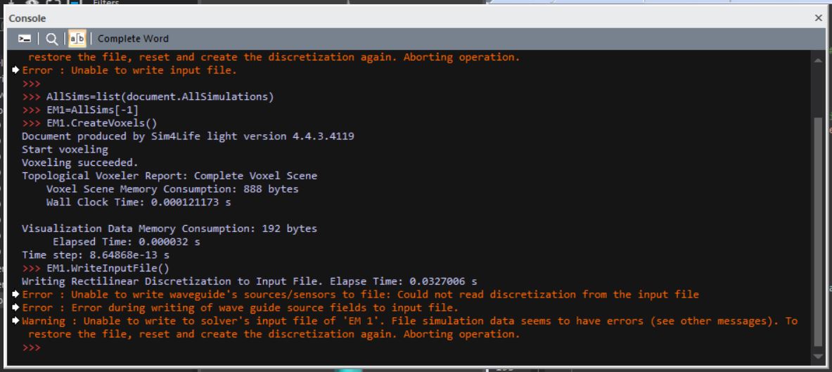
  • Error: FDTD multiport when writing input file

    2
    4
    0 Votes
    2 Posts
    1k Views
    S
    Hi, Have you tried to run this simulation as "Single FDTD", instead of "Multiport"? You can convert from one type to the other by right-clicking on the simulation and choosing "Clone As" -> "Single FDTD". I am not sure Multiport simulations have support for waveguide sources (and you have only one such source, so Single FDTD should anyway be what you need).
  • How do I calculate the total deposited power

    4
    0 Votes
    4 Posts
    2k Views
    A
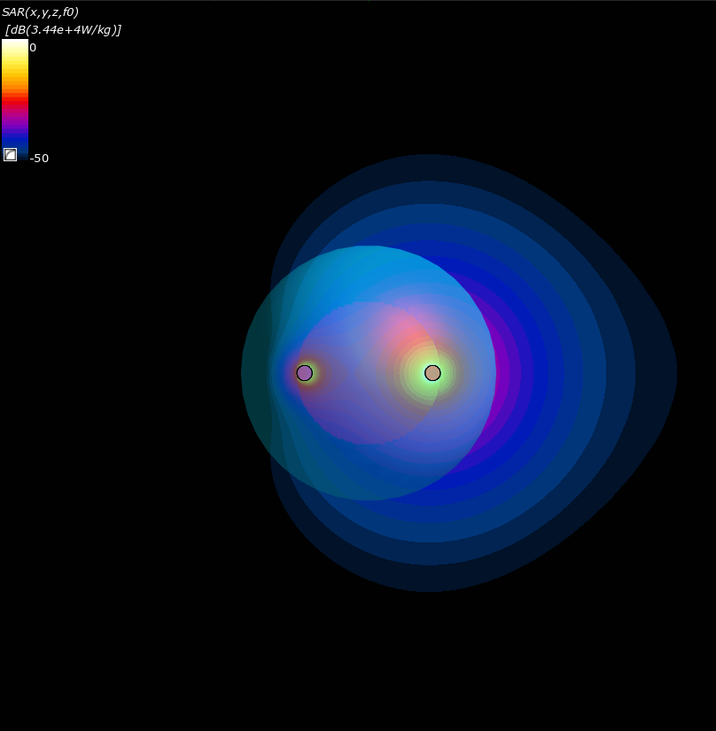
    Next to the "Statistics"-button you can see a "Viewers"-button, which has a wide variety of options on how to visualize your data. It includes slice viewers where you can see the SAR-distribution of an arbitrary plane, a histogram plot option, and much more.
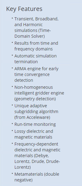
  • Simulation for Metamaterials

    1
    3
    0 Votes
    1 Posts
    805 Views
    No one has replied