Hi,
There is most likely an error due to a sanity check, since you appear to have lossy tissues in your simulation and the Magneto Static Vector Potential solver does not account for those losses. Having a ferrous core, however, you do need to use that solver.
The trick is to chain 2 simulations: one that solves the magnetic vector potential (A), and one that uses this A as a source term to determine the induced electric field (this time accounting for losses). The key is to remove the lossy tissues from the first simulation (only metallic or ferrous materials play a role anyhow).
I would recommend you have a look at the LF tutorial called "Wireless Power Transfer: Exposure Assessment", since it uses the same technique.
In addition, it seems that "The solver may have run out of RAM"... I would therefore check the RAM usage to make sure it's not going beyond your resources. Note that using the technique above allows you to have two different resolutions: one optimized to properly resolve the coil, the other to resolve the tissues (as long as the domain sizes of the first simulation is large enough to include that of the second). This usually leads to smaller grid sizes, thereby reducing the RAM usage...