Hi!
In all the tutorial python scripts this is shown. Within the python scripter you can click on the folder icon and choose "Open Example Script". There you will find lots of python scripts, that show how this is done.
Here a small excerpt from the script "tutorial_emlf_parallel_plate.py":
sim = CreateSimulation()
s4l_v1.document.AllSimulations.Add(sim)
sim.UpdateGrid()
sim.CreateVoxels(path)
sim.RunSimulation(wait=True)
I suggest always creating a simulation, and an analysis function, that is then called in the RunTutorial function. It's best to then also create a main:
def RunTutorial( path ):
import s4l_v1.document
s4l_v1.document.New()
CreateModel()
sim = CreateSimulation()
s4l_v1.document.AllSimulations.Add(sim)
sim.UpdateGrid()
sim.CreateVoxels(path)
sim.RunSimulation(wait=True)
AnalyzeSimulation(sim)
def main(data_path=None, project_dir=None):
"""
data_path = path to a folder that contains data for this simulation (e.g. model files)
project_dir = path to a folder where this project and its results will be saved
"""
import sys
import os
print("Python ", sys.version)
print("Running in ", os.getcwd(), "@", os.environ['COMPUTERNAME'])
if project_dir is None:
project_dir = os.path.expanduser(os.path.join('~', 'Documents', 's4l_python_tutorials') )
if not os.path.exists(project_dir):
os.makedirs(project_dir)
fname = os.path.splitext(os.path.basename(_CFILE))[0] + '.smash'
project_path = os.path.join(project_dir, fname)
RunTutorial( project_path )
if __name__ == '__main__':
main()