Hi @fangohr,
this is a very important question, especially considering the strong electrical anisotropy of muscle tissue.
Unfortunately, the whole-body anatomical models provided with Sim4Life do not include DTI information that could be used to assign anisotropic properties. Therefore, if you want to model tissue anisotropy, alternative approaches are required. Some of these may be reasonable when the stimulation is regional, i.e. limited to a small number of muscles.
In principle, Sim4Life allows you to model heterogeneous tissue anisotropy in two main ways.
1) Using subject-specific DTI data
If you are working with a personalized model (e.g. a head model) and have subject-specific DWI data, you can proceed as follows:
a. Reconstruct the DTI data from the DWI, bvec, and bval files (all standard outputs of MRI DTI).
b. Convert the DTI into a conductivity tensor field using the Tuch model [1]
Both steps are fully implemented in Sim4Life. Step (1) is performed via the Python API (please refer to the “Anisotropic Conductivity Tutorial” in the Examples section), while step (2) can be executed either through the Python API or directly in the GUI.
The attached animation shows how processed DTI data can be converted into tissue anisotropy data structure using the Tuch approach, and assigned to WM conductivity.
2) Without DTI data (assumption-based approach) - Using an E-field distribution & Cylindrical Tensor Model
If DTI data are not available, an alternative approach is possible, but its validity is entirely your responsibility.
Sim4Life allows you to create a conductivity tensor field from a 3D vector field by assuming cylindrical symmetry of the conductivity tensor. In this case, the principal tensor direction is assigned according to the local direction of the vector field, and only the longitudinal (parallel to the fibers) and radial (perpendicular to the fibers) conductivities need to be specified (you can find these values in the IT'IS LF Database (https://itis.swiss/virtual-population/tissue-properties/database/low-frequency-conductivity/)
The input vector field can be, for example, an E-field computed with any EM solver in Sim4Life, or a vector field generated via the Python API. One possible strategy would be to create an E-field aligned with the muscle fibers. This requires assumptions about muscle fiber organization — for instance, that fibers follow a diffusion-like process and extend from tendon to tendon. Under such assumptions, fiber directions could be approximated using an E-field computed with the QS-Ohmic Current solver, where the muscle is modeled as a homogeneous tissue and the tendons at the extremities act as Dirichlet boundary conditions.
Please note that this is not a ready-to-use recipe. This approach may be reasonable for certain muscles and unsuitable for others, and it represents a strong simplification of the underlying physiology. You will need to define a plausible fiber model and then use Sim4Life to test and validate your assumptions.
I hope this helps. If you need further or more specific assistance, please feel free to write again or contact the Sim4Life support team directly.
All the best,
Antonino
[1] Tuch, D. S., et al. Conductivity tensor mapping of the human brain using diffusion tensor MRI. Proceedings of the National Academy of Sciences, 98(20), 11697–11701 (2001).
[image: 1769594990533-anisotropy_from_dti_4.gif]